
RESEARCH ARTICLE
Data Detection in Single User Massive MIMO Using Re-Transmissions
K. Vasudevan*, K. Madhu, Shivani Singh
Article Information

Identifiers and Pagination:
Year: 2019Volume: 6
First Page: 15
Last Page: 26
Publisher Id: TOSIGPJ-6-15
DOI: 10.2174/1876825301906010015
Article History:
Received Date: 31/10/2018Revision Received Date: 28/1/2019
Acceptance Date: 22/02/2019
Electronic publication date: 29/03/2019
Collection year: 2019
open-access license: This is an open access article distributed under the terms of the Creative Commons Attribution 4.0 International Public License (CC-BY 4.0), a copy of which is available at: https://creativecommons.org/licenses/by/4.0/legalcode. This license permits unrestricted use, distribution, and reproduction in any medium, provided the original author and source are credited.
Abstract
Background:
Single user Massive Multiple Input Multiple Output (MIMO) can be used to increase the spectral efficiency since the data is transmitted simultaneously from a large number of antennas located at both the base station and mobile. It is feasible to have a large number of antennas in the mobile, in the millimeter wave frequencies. However, the major drawback of single user massive MIMO is the high complexity of data recovery at the receiver.
Methods:
In this work, we propose a low complexity method of data detection with the help of re-transmissions. A turbo code is used to improve the Bit-Error-Rate (BER).
Results and Conclusion:
Simulation results indicate a significant improvement in BER with just two re-transmissions as compared to the single transmission case. We also show that the minimum average SNR per bit required for error-free propagation over a massive MIMO channel with re-transmissions is identical to that of the Additive White Gaussian Noise (AWGN) channel, which is equal to -1.6 dB.
1. INTRODUCTION
The main idea behind single user massive Multiple Input Multiple Output (MIMO) [1-7] is to increase the bit rate between the transmitter and receiver over a wireless channel. This is made possible by sending the bits or symbols (groups of bits) simultaneously from a large number of transmit antennas. The signal at each receive antenna is a linear combination of the bits or symbols sent from all the transmit antennas plus Additive White Gaussian Noise (AWGN). We assume that the carrier frequency offset is absent or has been accurately estimated and canceled with the help of training symbols (preamble) [8-12]. The task of the receiver is to estimate the transmitted bits or symbols, from the signals in all the receive antennas. Note that it is possible to have a large number of antennas in both the base station and the mobile, in millimeter wave frequencies [13-21], due to the small size of the antennas.
If both the transmitter and receiver have N antennas and the symbols are drawn from an M-ary constellation, the complexity of the Maximum Likelihood (ML) detector would be MN, since it exhaustively searches all possible symbol combina-tions. Clearly, the ML detector is impractical. On the other hand, the “zero-forcing” solution is to multiply the received signal vector by the inverse of the channel matrix, which eliminates the interference from the other symbols. However, the computational complexity of inversion of the N×N channel matrix, for large values of N, does not make this approach attractive. Moreover, when the noise vector is multiplied by the inverse of the channel matrix, it usually results in noise enhan-cement, leading to poor Bit-Error-Rate (BER) performance.
In [22], a split pre-conditioned conjugate gradient method for data detection in massive MIMO is proposed. A low-complexity soft-output data detection scheme based on Jacobi method is presented in [23], Near-optimal data detection based on steepest descent and the Jacobi method is presented in [24]. Matrix inversion based on Newton iteration for large antenna arrays is given in [25] Subspace methods of data detection in MIMO are presented in [26, 27]. Data detection in large scale MIMO systems using Successive Interference Cancellation (SIC) is given in [28]. MIMO data detection in the presence of phase noise is given in [29]. Detection of LDPC coded symbols in MIMO systems is discussed in [30]. Decoding of convolutional codes in MIMO systems is presented in [31]. Decoding of polar codes in MIMO systems is given in [32]. Sphere decoding procedures for the detection of symbols in MIMO systems are discussed in [33-35]. Large scale MIMO detection algorithms are presented in [36]. Multiuser detection in massive MIMO with power efficient low-resolution ADCs is given in [37]. Joint ML detection and channel estimation in multiuser massive MIMO are presented in [38]. Detection of turbo coded offset QPSK in the presence of frequency and clock offsets and AWGN is presented in [39, 40]. Channel estimation in large antenna systems is given in [41-43]. Channel-aware data fusion for massive MIMO, in the context of Wireless Sensor Networks (WSNs), is proposed in [44].
In all the papers in the literature, on the topic of data detection in massive MIMO, the main lacuna has been in the definition of (or rather the lack of it) the signal-to-noise ratio (SNR). In fact, even the operating SNR of a mobile phone is not known [9-12, 45]. It may be noted that mobile phones indicate a typical signal strength of -100 dBm (10-10 milliwatt). However, this is not the SNR. In this work, we use the SNR per bit as the performance measure, since there is a lower bound on the SNR per bit for error-free transmission over any type of channel, which is -1.6 dB [11, 12]. The so-called “capacity” of MIMO channels has been derived earlier in [46-49]. However, the channel capacity is derived differently in [11], [12] and in this work. Therefore, the question naturally arises: are the present-day wireless telecommunication systems operating anywhere near the channel capacity? This question assumes significance in the context of 5G wireless communications where not only humans, but also machines and devices would be connected to the internet to form the Internet of Things (IoT) [50]. Hence, in order to minimize the global energy consumption due to IoT, it is necessary for each device to operate as close to the minimum average SNR per bit for error-free transmission, as possible [9-12], [45, 51]. Finally, one might ask the question: is it not possible to increase the bit-rate by increasing the size of the constellation, and using just one transmit and receive antenna? The answer is: increasing the size of the constellation increases the peak-to-Average Power Ratio (PAPR), which poses a problem for the Radio Frequency (RF) front end amplifiers, in terms of the dynamic range. In other words, a large PAPR requires a large dynamic range, which translates to low power efficiency, for the RF amplifiers [52].
In this work, we re-transmit a symbol Nrt times and then take the average, which results in a lower interference power compared to the single transmission case. Perfect Channel State Information (CSI) is assumed. The BER is improved with the help of a turbo code. This paper is organized as follows. Section 2 describes the system model. The receiver design is presented in Section 3. The Bit-Error-Rate (BER) results from computer simulations are given in Section 4. Finally, Section 5 presents the conclusion and future work.
2. SYSTEM MODEL
Consider the system model in Fig. (1). The data bits are organized into frames of length Ld1 bits. The Recursive Systematic Convolutional (RSC) encoders 1 and 2 encode the data bits into Quadrature Phase Shift Keyed (QPSK) symbols having a total length of Ld. We assume a MIMO system with N transmit and N receive antennas. We also assume that Ld /N is an integer, where Ld = 2Ld1 as shown in Fig. (1). The Ld QPSK symbols are transmitted, N symbols at a time, from the N transmit antennas.
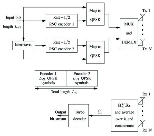 |
Fig. (1). System model. |
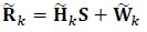
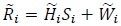
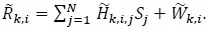
The received signal in the kth (0 ≤ k ≤ Nrt-1, k is an integer), re-transmission is given by [11, 12]
 |
(1) |
where  is the received vector,
  is the channel matrix and
  is the Additive White Gaussian Noise (AWGN) vector. The transmitted symbol vector is
  , whose elements are drawn from an M-ary conste-llation. Boldface letters denote vectors or matrices. Complex quantities are denoted by a tilde. However, tilde is not used for complex symbols S. The elements of
  are statistically independent with zero mean and variance per dimension equal to
  , that is
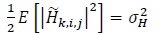 |
(2) |
where E [·] denotes the expectation operator [53, 54],  denotes the element in the ith row and jth column of . Similarly, the elements of
  are statistically independent with zero mean and variance per dimension equal to
  , that is
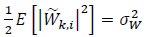 |
(3) |
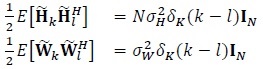
where  denotes the element in the ith row of . The real and imaginary parts of and are also assumed to be independent. The channel and noise are assumed to be independent across re-transmissions, that is
 |
(4) |
where the superscript (·) denotes Hermitian (conjugate transpose of a matrix), IN is an N × N identity matrix and δk(m)(m is an integer) is the Kronecker delta function defined by
 |
(5) |
The receiver is assumed to have perfect knowledge of .
3. RECEIVER
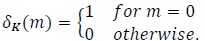
In this section, we describe the procedure for detecting S given the received signal  in (1). Consider
 |
(6) |
where
 |
(7) |
Observe that similar to (4) we have
 |
(8) |
However,
 |
(9) |
The main aim of this work is to replace the expectation operator in (8) by time-averaging, in the form of re-transmi-ssions, so that the right-hand-side of (8) is approximately satisfied.
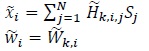
Now the ith element of  in (6) is
 |
(10) |
where
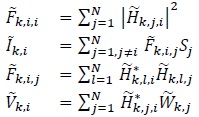 |
(11) |
where it is understood that  is real-valued. Note that for large values of N,
  and
and  are Gaussian distributed due to the central limit theorem [53]. Moreover, since Si and are independent, and are uncorrelated, that is
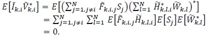 |
(12) |
Let
 |
(13) |
|
where |
 |
(14) |
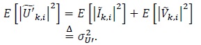
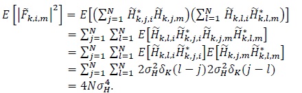
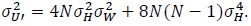
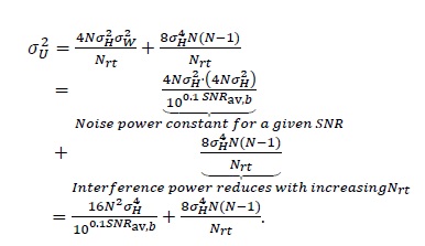
The noise power is
 |
(15) |
|
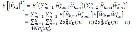
where we have used the sifting property of the Kronecker delta function. The interference power is |
 |
(16) |
where
 |
(17) |
and
 |
(18) |
Substituting (15) and (16) in (14) we get
 |
(19) |
Consider
 |
(20) |
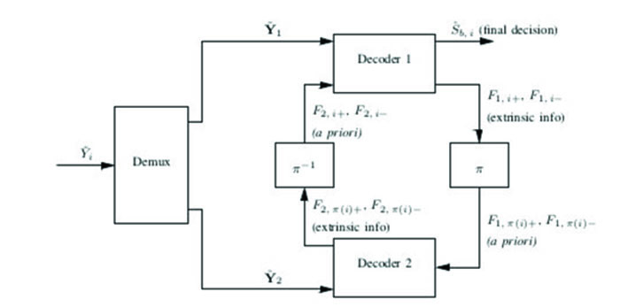 |
Fig. (2). Turbo decoder. |
where  is defined in (10) and
 |
(21) |
Note that Fi in (21) is real-valued. Since  is indepen-dent over k we have
 |
(22) |
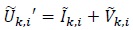
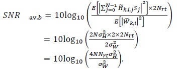
In other words, the interference plus noise power reduces due to averaging. The average signal-to-noise ratio per bit in decibels is defined as [11, 12] (see also the appendix)
 |
(23) |
From (23) we can write
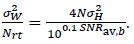 |
(24) |
Substituting (24) in (22) we get
 |
(25) |
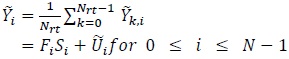
After concatenation, the signal  and Fi,i in (20) for 0 ≤ i ≤ Ld -1 is sent to the turbo decoder [54], as explained below.
3.1. Turbo Decoding - The BCJR Algorithm
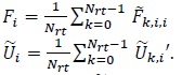
The block diagram of the turbo decoder is depicted in Fig. (2). Note that
 |
(26) |
The BCJR algorithm has the following components:
- The forward recursion
- The backward recursion
- The computation of the extrinsic information and the final a posteriori probabilities.
Let  denote the number of states in the encoder trellis. Let
  denote the set of states that diverge from state
  , for 0 ≤ ≤ - 1. For example
 |
(27) |
implies that states 0 and 3 can be reached from state 0. Similarly, let Cn denote the set of states that converge to state . Let αi,n denote the forward Sum-Of-Products (SOP) at time i (0 ≤ i ≤ Ld1 -2) at state . Then the forward SOP for decoder 1 can be recursively computed as follows (forward recursion) [54]
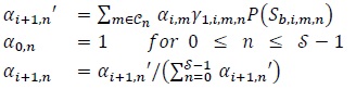 |
(28) |
where
 |
(29) |
denotes the a priori probability of the systematic (data) bit corresponding to the transition from state m to state , at decoder 1 at time i, obtained from the 2nd decoder at time l, after de-interleaving, that is i =π-1(l) for some 0 ≤ l ≤ Ld -1, l ≠ i and
 |
(30) |
where Sm,n denotes the coded QPSK symbol corresponding to the transition from state m to n in the trellis. The normalization step in the last equation of (28) is done to prevent numerical instabilities.
Let βi,n denote the backward SOP at time i (1 ≤ i ≤ Ld1-1) at state (0 ≤ ≤ - 1). Then the recursion for the backward SOP (backward recursion) at decoder 1 can be written as:
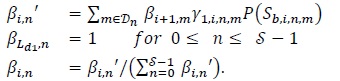 |
(31) |
Once again, the normalization step in the last equation (31) is done to prevent numerical instabilities.
Let  denote the state that is reached from state when the input symbol is +1. Similarly, let
  denote the state that can be reached from state when the input symbol is -1. Then the extrinsic information from decoder 1 to 2 is calculated as follows for 0 ≤ i ≤ Ld1-1
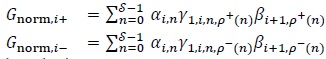 |
(32) |
which is further normalized to obtain
 |
(33) |
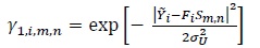
Equations (28), (31), (32) and (33) constitute the MAP recursions for the first decoder. The MAP recursions for the second decoder are similar excepting that γ1,i,m,n is replaced by
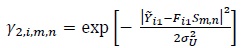 |
(34) |
where  and Fi 1 are obtained by concatenating and Fi,i in (20) and
 |
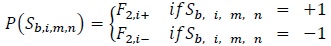
(35) |
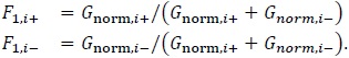
and F1,i+, F1,i- in (33) is replaced by F2,1+ and F2,i- respectively (Fig. (2)).
After several iterations, the final a posteriori probabilities of the ith data bit obtained at the output of the first decoder is computed as (for 0 ≤ i ≤Ld1 - 1):
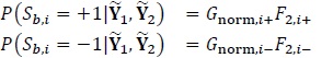 |
(36) |
where again F2,k+ and F2,k- denote the a priori probabilities obtained at the output of the second decoder (after de-interleaving) in the previous iteration. The final estimate of the ith data bit is given as Fig. (2):
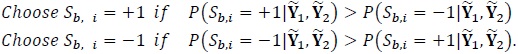 |
(37) |
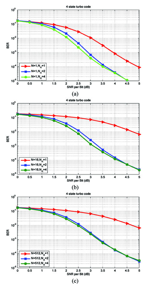 |
Fig. (3). Results for the 4-state turbo code in (38). |
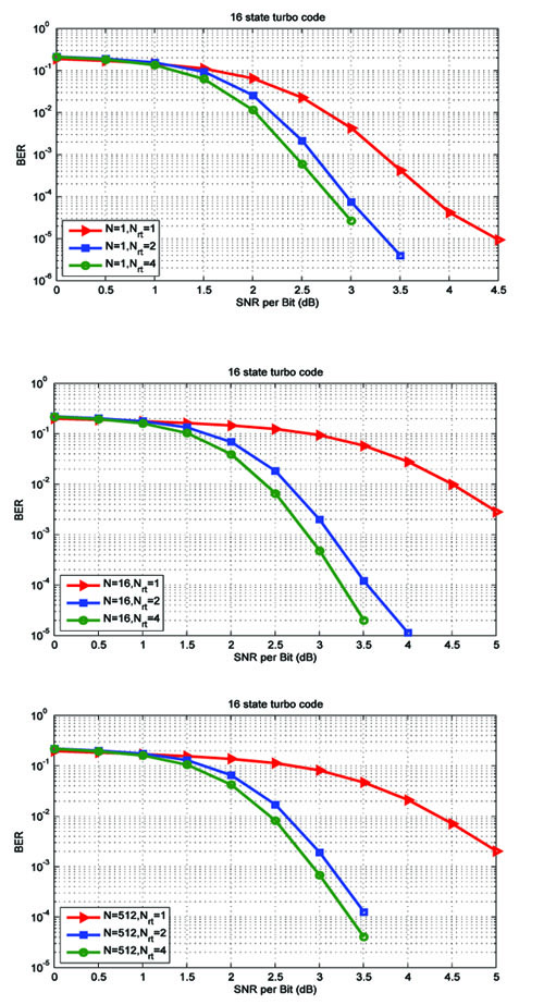 |
Fig. (4). Results for the 16-state turbo code in (40). |
| Parameter | Value |
|---|---|
| Ld1 | 512 |
| Ld | 1024 |
| N | 1, 16, 512 |
| Nrt | 1, 2, 4 |
| No. of frames simulated | 105, 106 |
| No. of turbo decoders iterations | 8 |
Note that:
- One iteration involves decoder 1 followed by decoder 2.
- Since the terms αi,n and βi,n depend on F2,i+, F2,i- for decoder 1, and F1,i+, F1,i- for decoder 2, they have to be recomputed for every decoder in every iteration accor-ding to (28) and (31) respectively.
In the computer simulations, robust turbo decoding [9] has been incorporated, that is, the exponent in (30) and (34) is normalized to the range [-30,0].
4. SIMULATION RESULTS AND DISCUSSION
In this section, we present the results from computer simulations. The simulation parameters are presented in Table 1.
At high SNR, the number of frames simulated is 106, whereas for low and medium SNR, the number of frames simulated is 105.
In Fig. (3), we present the simulation results for a 4-state turbo code with generating matrix given by
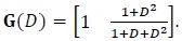 |
(38) |
From Figs. (3a-3c) we see the following.
1. There is no significant degradation in the BER performance due to the increase in the number of antennas (N), for a given number of re-transmissions Nrt > 1. For example, with Nrt = 2 and N = 16, a BER of 10-4 is attained at an SNR per bit of 4 dB, whereas the same BER is attained at an SNR per bit of 4.25 dB for N = 512 - this is just a 0.25 dB degradation in performance. Observe that the spectral efficiency with N = 16 antennas and Nrt = 2 re-transmissions, is 4 bits/transmission or 4 bits/sec/Hz, since each QPSK symbol carries 1/4 bits of information (see appendix). However, the spectral efficiency with N = 512 antennas and Nrt = 2 re-transmissions is 128 bits/sec/Hz. In other words, an increase in the spectral efficiency by a factor of 32 results in only a 0.25 dB degradation in the BER performance.
2. With Nrt = 2, there is significant improvement in BER performance compared to Nrt = 1, for all values of N. However the BER performance with Nrt = 4 is comparable to Nrt = 2. This is because, with increasing Nrt the BER is limited by the variance of the noise term in (25), even though the variance of the interference term gets reduced due to averaging.
3. Note that when N = 1, the interference is zero and only noise is present. We see from Fig. (3a) that there is a significant improvement in performance for Nrt = 2, compared to Nrt = 1. This can be attributed to the fact that Fi in (21) contains two positive terms (independent Rayleigh distributed random variables) for Nrt = 2 compared to Nrt = 1. Hence, the probability that both terms are simultaneously close to zero, is small.
4. It is interesting to compare the case N = Nrt = 1 in Fig. (3a) with Figure 12 in [12] with Nr = 1. Both systems are identical, in terms of the received signal model, that is
 |
(39) |
where i denotes the time index. In this work, we obtain a BER of 10-4 at an average SNR per bit of 5 dB, whereas in [12] we obtain the same BER at an average SNR per bit of just 2.25 dB. What could be the reason for this difference? The answer lies in the computation of gammas. In this work, the gammas are computed using (30) and (34), which is sub-optimum compared to (66) in [12]. This is because, the noise term  in (20) is equal to
  , which is not even Gaussian (recall that is Gaussian for large values of N due to the central limit theorem). However, in this work, we are assuming that is Gaussian, for N = 1.
In Fig. (4), we present the simulation results for a 16-state turbo code with generating matrix given by [54]
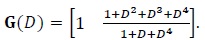 |
(40) |
We observe the following in Figs. (4a-4c):
1. There is again a significant improvement in BER performance for Nrt = 2, compared to Nrt = 1. However, the improvement in BER for Nrt = 4 is not much, compared to Nrt = 2.
2. Comparing Figs. (3 and 4), with N = 16 and Nrt = 2, the encoder in (40) gives only a 0.5 dB improvement at a BER of 10-4, over the encoder in (38).
3. Comparing Figs. (3 and 4), with N = 512 and Nrt = 2, the encoder in (40) gives only a 0.75 dB improvement at a BER of 10-4, over the encoder in (38). These results indicate that this may not be the best 16-state turbo code.
CONCLUSION
We have shown by analysis as well as computer simula-tions that, as the number of retransmissions increase, the BER decreases. There is little improvement by using a 16-state turbo code as compared to the 4-state code, in terms of the BER. Perhaps, this may not be the best 16-state turbo code. Future work could be to use iterative interference cancellation with no re-transmissions since the re-transmissions reduce the spectral efficiency. Estimating the N×N channel matrix is also a good topic for future research.
We derive the minimum average SNR per bit required for error-free propagation over a massive MIMO channel with re-transmissions. Consider the signal
 |
(41) |
where the subscript i denotes the time index,  is the transmitted signal (message) and
  denotes samples of zero-mean noise, not necessarily Gaussian, with variance per dimension equal to σw2. All the terms in (41) are complex-valued or two-dimensional. Here the term “dimension” refers to a communication link between the transmitter and the receiver carrying only real-valued signals [11, 12] The number of bits per transmission, defined as the channel capacity, is given by [11, 12, 55]
 |
(42) |
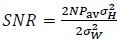
over a complex dimension, where the average SNR is given by
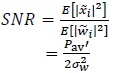 |
(43) |
over a complex dimension. Recall that (42) gives the minimum SNR for the error-free propagation of C bits.
Proposition 6.1 The channel capacity is additive over the number of complex dimensions. In other words, the channel capacity over N complex dimensions, is equal to the sum of the capacities over each complex dimension, provided the information is independent across the complex dimensions [9], [11, 12]. Independence of information also implies that, the bits transmitted over one complex dimension is not the interleaved version of the bits transmitted over any other complex dimension.
Proposition 6.2 Conversely, if C bits per transmission are sent over N complex dimensions, it seems reasonable to assume that each complex dimension receives C/N bits per transmission [9, 11, 12].
The reasoning for Proposition 6.2 is as follows. We assume that a “bit” denotes “information”. Now, if each of the N antennas (complex dimensions) receive the “same” C bits of information, then we might as well have only one antenna, since the other antennas are not yielding any additional information. On the other hand, if each of the N antennas receive “different” C bits of information, then we end up receiving more information (CN bits) than what we transmit (C bits), which is not possible. Therefore, we assume that each complex dimension receives C/N bits of “different” information.
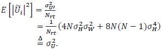
Observe that the average SNR in (43) is not the average SNR per bit over a complex dimension. In order to compute the average SNR per bit, we note from Fig. (1) that each data bit generates two QPSK symbols, and each QPSK symbol is repeated Nrt times. Therefore, from Proposition 6.2, each QPSK symbol carries 1⁄(2Nrt) bits of information. The information sent in one transmission is N⁄(2Nrt) bits, from the N transmit antennas (Proposition 6.1). The information in each receive antenna in one transmission over a complex dimension is (Proposition 6.2):
 |
(44) |
which is identical to the channel capacity in (42).
Let us now consider the ith element of in (1). We have
 |
(45) |
Now, if we substitute
 |
(46) |
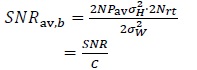
in (41), the channel capacity remains unchanged, as given in (42), with SNR equal to
 |
(47) |
where
 and Pav are defined in (2), (3) and (17) respectively. However, the information contained in
  in (45) is 1⁄(2 Nrt) bits (see (44)), hence the SNR in (47) is for 1⁄(2 Nrt) bits. Therefore, the SNR per bit is
 |
(48) |
where we have used (44). Substituting (48) in (42) we get
 |
(49) |
|
over a complex dimension. Re-arranging terms in (49) we get |
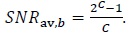 |
(50) |
Thus (50) implies that as  which is the minimum average SNR per bit required for error-free propagation over a massive MIMO channel, with re-transmissions. Just as in the case of turbo codes, it may not be necessary for C to approach zero, in order to attain the channel capacity.
NOTES
1 The authors are with the Department of Electrical Engineering, Indian Institute of Technology Kanpur, 208016, India. email:vasu@iitk.ac.in, madhukasina508@gmail.com, shivanis@iitk.ac.in
CONSENT FOR PUBLICATION
Not applicable.
CONFLICT OF INTEREST
The authors declares no conflict of interest, financial or otherwise.
ACKNOWLEDGEMENTS
Declared none.
REFERENCES
| [1] | Foschini GJ. Layered space-time architecture for wireless communication in a fading environment when using multi-element antennas. Bell Labs Tech J 1996; 1: 41-59. |
| [2] | Lu L, Li GY, Swindlehurst AL, Ashikhmin A, Zhang R. An overview of massive MIMO:Benefits and challenges. IEEE J Sel Top Signal Process 2014; 8: 742-58. |
| [3] | Wolniansky PW, Foschini GJ, Golden GD, Valenzuela RA. 1998; V-BLAST: An architecture for realizing very high data rates over the rich-scattering wireless channel. 1998 URSI International Symposium on Signals, Systems, and Electronics Conference Proceedings (Cat No98EX167) 295-300. |
| [4] | Rusek F, Persson D, Lau BK, et al. Scaling up MIMO: Opportunities and challenges with very large arrays. IEEE Signal Process Mag 2013; 30: 40-60. |
| [5] | Larsson EG, Edfors O, Tufvesson F, Marzetta TL. Massive MIMO for next generation wireless systems. IEEE Commun Mag 2014; 52: 186-95. |
| [6] | Gozalvez J. Samsung electronics sets 5G speed record at 7.5 Gb/s. IEEE Veh Technol Mag 2015; 10: 12-6. [Mobile Radio]. |
| [7] | Marzetta TL. Massive MIMO: An Introduction. Bell Labs Tech J 2015; 20: 11-22. |
| [8] | Vasudevan K. Coherent detection of turbo coded OFDM signals transmitted through frequency selective Rayleigh fading channels In: In Signal Processing, Computing and Control (ISPCC), 2013 IEEE International Conference ; 2013; pp. 2013; 1-6. |
| [9] | Vasudevan K. Coherent detection of turbo-coded OFDM signals transmitted through frequency selective rayleigh fading channels with receiver diversity and increased throughput. Wirel Pers Commun 2015; 82: 1623-42. |
| [10] | Vasudevan K. Coherent detection of turbo-coded OFDM signals transmitted through frequency selective rayleigh fading channels with receiver diversity and increased throughput 2015b. CoRR abs/1511.00776 |
| [11] | Vasudevan K. 2016; Coherent Turbo Coded MIMO OFDM In ICWMC 2016 The 12thInternational Conference on Wireless and Mobile Communications ; 2016; pp. 91-9. |
| [12] | Vasudevan K. Near capacity signaling over fading channels using coherent turbo coded OFDM and massive MIMO. Int J Adv Telecom 2017; 10: 22-37. [Online]. |
| [13] | Pi Z, Khan F. An introduction to millimeter-wave mobile broadband systems. IEEE Commun Mag 2011; 49: 101-7. |
| [14] | Rappaport TS, Sun S, Mayzus R, et al. Millimeter wave mobile communications for 5G Cellular: It will work! IEEE Access 2013; 1: 335-49. |
| [15] | Roh W, Seol JY, Park J, et al. Millimeterwave beamforming as an enabling technology for 5G cellular communications: Theoretical feasibility and prototype results. IEEE Commun Mag 2014; 52: 106-13. |
| [16] | Andrews JG, Buzzi S, Choi W, et al. What will 5G be? IEEE J Sel Areas Comm 2014; 32: 1065-82. |
| [17] | Rappaport TS, Roh W, Cheun K. Mobile’s millimeter-wave makeover. IEEE Spectr 2014; 51: 34-58. |
| [18] | Wu T, Rappaport TS, Collins CM. Safe for generations to come. IEEE Microw Mag 2015; 16(2): 65-84. |
| [19] | Niknam S, Nasir AA, Mehrpouyan H, Natarajan B. A multiband OFDMA heterogeneous network for millimeter wave 5G wireless applications. IEEE Access 2016; 4: 5640-8. |
| [20] | Wong KL, Tsai CY, Lu JY, Chian DM, Li WY. Compact eight MIMO antennas for 5G smartphones and their MIMO capacity verification 2016 ; 1054-6. |
| [21] | Buzzi S, D’Andrea C. 2016; Doubly massive mmWave MIMO systems: Using very large antenna arrays at both transmitter and receiver. 2016 IEEE Global Communications Conference (GLOBECOM) 1-6. |
| [22] | Jin J, Xue Y, Ueng YL, You X, Zhang C. 2017; A split pre-conditioned conjugate gradient method for massive MIMO detection. 2017 IEEE International Workshop on Signal Processing Systems (SiPS) 1-6. |
| [23] | Jiang F, Li C, Gong Z. 2017; A low complexity soft-output data detection scheme based on Jacobi method for massive MIMO uplink transmission. 2017 IEEE International Conference on Communications (ICC) 1-5. |
| [24] | Qin X, Yan Z, He G. A near-optimal detection scheme based on joint steepest descent and jacobi method for uplink massive MIMO systems. IEEE Commun Lett 2016; 20: 276-9. |
| [25] | Tang C, Liu C, Yuan L, Xing Z. High precision low complexity matrix inversion based on newton iteration for data detection in the massive MIMO. IEEE Commun Lett 2016; 20: 490-3. |
| [26] | Chen Y, ten Brink S. 2011.Near-capacity MIMO subspace detection. In 2011 IEEE 22nd International Symposium on Personal, Indoor and Mobile Radio Communications pp. 1733–1737 |
| [27] | Wang X, ten Brink S. 2017; Iterative MIMO Subspace Detection Based on Parallel Interference Cancellation. In 2017 IEEE Wireless Communications and Networking Conference (WCNC) 1-6. |
| [28] | Mandloi M, Hussain MA, Bhatia V. Improved multiple feedback successive interference cancellation algorithms for near-optimal MIMO detection. IET Commun 2017; 11: 150-9. |
| [29] | Datta T, Yang S. 2015.Improving MIMO detection performance in presence of phase noise using norm difference criterion. In 53rd Annual Allerton Conference on Communication, Control, and Computing (Allerton) pp. 286–292, 2015 |
| [30] | Jing S, Yang J, Wang Z, You X, Zhang C. 2017; Algorithm and architecture for joint detection and decoding for MIMO with LDPC codes. 2017 IEEE International Symposium on Circuits and Systems (ISCAS) 1-4. |
| [31] | Sukumar CP, Shen CA, Eltawil AM. Joint detection and decoding for MIMO systems using convolutional codes: Algorithm and VLSI architecture. IEEE Trans Circuits Syst I Regul Pap 2012; 59: 1919-31. |
| [32] | Yang J, Zhang C, Song W, Xu S, You X. 2016; Joint detection and decoding for MIMO systems with polar codes. 2016 IEEE International Symposium on Circuits and Systems (ISCAS) 161-4. |
| [33] | Guo Z, Nilsson P. Algorithm and implementation of the K-best sphere decoding for MIMO detection. IEEE J Sel Areas Comm 2006; 24: 491-503. |
| [34] | Ju C, Ma J, Tian C, He G. 2012; VLSI implementation of an 855 Mbps high performance softoutput K-Best MIMO detector. 2012 IEEE International Symposium on Circuits and Systems 2849-52. |
| [35] | Sah AK, Chaturvedi AK. An MMP-based approach for detection in large MIMO systems using sphere decoding. IEEE Wirel Commun Lett 2017; 6: 158-61. |
| [36] | Wu M, Yin B, Wang G, Dick C, Cavallaro JR, Studer C. Large-scale MIMO detection for 3GPP LTE: Algorithms and FPGA implementations. IEEE J Sel Top Signal Process 2014; 8: 916-29. |
| [37] | Wang S, Li Y, Wang J. Multiuser detection in massive spatial modulation MIMO with low-resolution ADCs. IEEE Trans Wirel Commun 2015; 14: 2156-68. |
| [38] | Choi J, Mo J, Heath RW. Near maximum-likelihood detector and channel estimator for uplink multiuser massive MIMO systems with one-bit ADCs. IEEE Trans Commun 2016; 64: 2005-18. |
| [39] | Vasudevan K. Iterative detection of turbo coded offset QPSK in the presence of frequency and clock offsets and AWGN. Signal, Image and Video Processing, Springer 2012; 6: 557-67. |
| [40] | Vasudevan K. Design and development of a burst acquisition system for geosynchronous satcom channels 2015. CoRR abs/1510.07106 |
| [41] | Ma J, Ping L. Data-aided channel estimation in large antenna systems. IEEE Trans Signal Process 2014; 62: 3111-24. |
| [42] | Shen W, Dai L, Gao Z, Wang Z. Spatially correlated channel estimation based on block iterative support detection for massive MIMO systems. Electron Lett 2015; 51: 587-8. |
| [43] | Peng Y, Li Y, Wang P. An enhanced channel estimation method for millimeter wave systems with massive antenna arrays. IEEE Commun Lett 2015; 19: 1592-5. |
| [44] | Ciuonzo D, Rossi PS, Dey S. Massive MIMO channel-aware decision fusion. IEEE Trans Signal Process 2015; 63: 604-19. |
| [45] | Vasudevan K. CWMC Special Session MAAZE - Wireless Communications: The march towards absolute zero- Editorial [Online] 2016. |
| [46] | Telatar E. Capacity of multiantenna gaussian channels. European Transactions on Telecommunications 1999; 10: 585-95. |
| [47] | Goldsmith A, Jafar SA, Jindal N, Vishwanath S. Capacity limits of MIMO channels. IEEE J Sel Areas Comm 2003; 21: 684-702. |
| [48] | Wang Y, Yue DW. Capacity of MIMO rayleigh fading channels in the presence of interference and receive correlation. IEEE Trans Vehicular Technol 2009; 58: 4398-405. |
| [49] | Benkhelifa F, Tall A, Rezki Z, Alouini MS. On the low SNR capacity of MIMO fading channels with imperfect channel state information. IEEE Trans Commun 2014; 62: 1921-30. |
| [50] | Agiwal M, Roy A, Saxena N. Next generation 5G wireless networks: A comprehensive survey. IEEE Comm Surv and Tutor 2016; 18: 1617-55. |
| [51] | Toward green and soft: a 5G perspective. IEEE Commun Mag 2014; 52: 66-73. |
| [52] | Halkias M. Integrated electronics. McGraw-Hill electrical and electronic engineering series Tata McGraw-Hill Publishing Company 2001. |
| [53] | Haykin S. Communication Systems 2nd ed. 1983. |
| [54] | Vasudevan K. 2010.Digital Communications and Signal Processing Second edition (CDROM included). Universities Press (India), Hyderabad www.universitiespress.com |
| [55] | Proakis JG, Salehi M. Fundamentals of Communication Systems 2005. |